分类模型归一化

零.导入所需库

import matplotlib as mpl
import matplotlib.pyplot as plt
%matplotlib inline
import numpy as np
import sklearn
import pandas as pd
import os
import sys
import time
import tensorflow as tf

from tensorflow import keras

print(tf.__version__)
print(sys.version_info)
for module in mpl, np, pd, sklearn, tf, keras:
    print(module.__name__, module.__version__)

2.0.0-alpha0
sys.version_info(major=3, minor=6, micro=13, releaselevel='final', serial=0)
matplotlib 3.3.4
numpy 1.16.2
pandas 1.1.5
sklearn 0.24.1
tensorflow 2.0.0-alpha0
tensorflow.python.keras.api._v2.keras 2.2.4-tf

一.加载数据集，划分训练集，测试集，验证集

fashion_mnist = keras.datasets.fashion_mnist
(x_train_all, y_train_all), (x_test, y_test) = fashion_mnist.load_data()
x_valid, x_train = x_train_all[:5000], x_train_all[5000:]
y_valid, y_train = y_train_all[:5000], y_train_all[5000:]

print(x_valid.shape, y_valid.shape)
print(x_train.shape, y_train.shape)
print(x_test.shape, y_test.shape)

(5000, 28, 28) (5000,)
(55000, 28, 28) (55000,)
(10000, 28, 28) (10000,)

二.数据归一化

print(np.max(x_train), np.min(x_train))

255 0

# 哪些机器学习算法不需要(需要)做归一化?
#  概率模型（树形模型）不需要归一化，因为它们不关心变量的值，而是关心变量的分布和变量之间的条件概率，
# 如决策树、RF。而像Adaboost、SVM、LR、Knn、KMeans之类的最优化问题就需要归一化。
# StandardScaler原理
# 作用：去均值和方差归一化。且是针对每一个特征维度来做的，而不是针对样本。 

# x = (x - u) / std
from sklearn.preprocessing import StandardScaler
scaler = StandardScaler()
# x_train: [None, 28, 28] -> [None, 784]
x_train_scaled = scaler.fit_transform(
    x_train.astype(np.float32).reshape(-1, 1)).reshape(-1, 28, 28)
x_valid_scaled = scaler.transform(
    x_valid.astype(np.float32).reshape(-1, 1)).reshape(-1, 28, 28)
x_test_scaled = scaler.transform(
    x_test.astype(np.float32).reshape(-1, 1)).reshape(-1, 28, 28)

print(np.max(x_train_scaled), np.min(x_train_scaled))

2.0231433 -0.8105136

四.构建模型

# tf.keras.models.Sequential()

"""
model = keras.models.Sequential()
model.add(keras.layers.Flatten(input_shape=[28, 28]))
model.add(keras.layers.Dense(300, activation="relu"))
model.add(keras.layers.Dense(100, activation="relu"))
model.add(keras.layers.Dense(10, activation="softmax"))
"""

model = keras.models.Sequential([
    keras.layers.Flatten(input_shape=[28, 28]),
    keras.layers.Dense(300, activation='relu'),
    keras.layers.Dense(100, activation='relu'),
    keras.layers.Dense(10, activation='softmax')
])

model.summary()

Model: "sequential"
_________________________________________________________________
Layer (type)                 Output Shape              Param #   
=================================================================
flatten (Flatten)            (None, 784)               0         
_________________________________________________________________
dense (Dense)                (None, 300)               235500    
_________________________________________________________________
dense_1 (Dense)              (None, 100)               30100     
_________________________________________________________________
dense_2 (Dense)              (None, 10)                1010      
=================================================================
Total params: 266,610
Trainable params: 266,610
Non-trainable params: 0
_________________________________________________________________

# relu: y = max(0, x)
# softmax: 将向量变成概率分布. x = [x1, x2, x3], 
#          y = [e^x1/sum, e^x2/sum, e^x3/sum], sum = e^x1 + e^x2 + e^x3

# reason for sparse: y->index. y->one_hot->[] 
model.compile(loss="sparse_categorical_crossentropy",
              optimizer = "sgd",
              metrics = ["accuracy"])

五.训练

history = model.fit(x_train_scaled, y_train, epochs=10,
                    validation_data=(x_valid_scaled, y_valid))

Train on 55000 samples, validate on 5000 samples
Epoch 1/10
55000/55000 [==============================] - 3s 55us/sample - loss: 0.9219 - accuracy: 0.6927 - val_loss: 0.6338 - val_accuracy: 0.7860
Epoch 2/10
55000/55000 [==============================] - 3s 53us/sample - loss: 0.5999 - accuracy: 0.7919 - val_loss: 0.5366 - val_accuracy: 0.8178
Epoch 3/10
55000/55000 [==============================] - 3s 54us/sample - loss: 0.5288 - accuracy: 0.8152 - val_loss: 0.4906 - val_accuracy: 0.8354
Epoch 4/10
55000/55000 [==============================] - 3s 54us/sample - loss: 0.4892 - accuracy: 0.8288 - val_loss: 0.4600 - val_accuracy: 0.8424
Epoch 5/10
55000/55000 [==============================] - 3s 53us/sample - loss: 0.4628 - accuracy: 0.8377 - val_loss: 0.4412 - val_accuracy: 0.8538
Epoch 6/10
55000/55000 [==============================] - 3s 53us/sample - loss: 0.4432 - accuracy: 0.8446 - val_loss: 0.4266 - val_accuracy: 0.8562
Epoch 7/10
55000/55000 [==============================] - 3s 55us/sample - loss: 0.4280 - accuracy: 0.8491 - val_loss: 0.4161 - val_accuracy: 0.8584
Epoch 8/10
55000/55000 [==============================] - 3s 55us/sample - loss: 0.4155 - accuracy: 0.8533 - val_loss: 0.4085 - val_accuracy: 0.8604
Epoch 9/10
55000/55000 [==============================] - 3s 53us/sample - loss: 0.4052 - accuracy: 0.8564 - val_loss: 0.4001 - val_accuracy: 0.8640
Epoch 10/10
55000/55000 [==============================] - 3s 52us/sample - loss: 0.3962 - accuracy: 0.8591 - val_loss: 0.3975 - val_accuracy: 0.8630

六.保存模型

save_model_name = './modelckpt/model-normalize.h5'
save_dir = './modelckpt/'
if not os.path.exists(save_dir):
    os.mkdir(save_dir)
model.save(save_model_name)

七.看下训练分布，验证分布

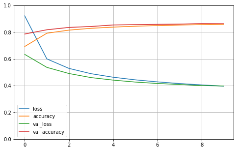
def plot_learning_curves(history):
    pd.DataFrame(history.history).plot(figsize=(8, 5))
    plt.grid(True)
    plt.gca().set_ylim(0, 1)
    plt.show()

plot_learning_curves(history)

​

​

model.evaluate(x_test_scaled, y_test)

10000/10000 [==============================] - 0s 28us/sample - loss: 0.4362 - accuracy: 0.8431





[0.43620746932029725, 0.8431]

test_loss, test_acc = model.evaluate(x_test_scaled, y_test)
print("准确率: %.4f，共测试了%d张图片 " % (test_acc, len(x_test)))

10000/10000 [==============================] - 0s 29us/sample - loss: 0.4362 - accuracy: 0.8431
准确率: 0.8431，共测试了10000张图片 

准确率84.31%